**Source: https://thlp-method.netlify.app/?en**
# METHOD FOR TRANSFORMING
# HIGHER-DIMENSIONAL LATTICES INTO THE PLANE
THLP: T = Transforming, H = Higher-Dimensional, L = Lattices, P = Plane
## A QUICK INTRODUCTION
On a first reading, it is not necessary to understand every detail of the
steps that follow. I suggest reading through them briefly and then asking
yourself: Did anything particularly complicated happen? Ideally, the answer
will be no.
It is best to begin by taking a look at the visualizations. Use the
Number Garden button in the title area to explore them interactively.
In Number Garden, double-click anywhere in the display or press N to
generate new examples. Sometimes it takes several attempts before a
particularly striking pattern appears. They emerge from the simple operations described
below, yet they do not appear as mere tiling patterns: they form remarkably
different visual worlds that nevertheless arise from the same defined
construction process.
Anyone wishing to reproduce the results on a computer will, of course, need
to understand the procedure in full. When implementing it on a computer, one
will then most likely encounter the real challenges.
Points are written as:
P = [x, y, ...]
In the following explanation, no distinction is made between a point and its
position vector. When P is called a vector, it means the vector from the
origin to the point P.
Imagine this:
In three-dimensional space, we allow three possible positions on each of the
x-, y-, and z-axes. On every axis, we may move one step in the negative
direction, remain at zero, or move one step in the positive direction:
x, y, z in {-1, 0, 1}
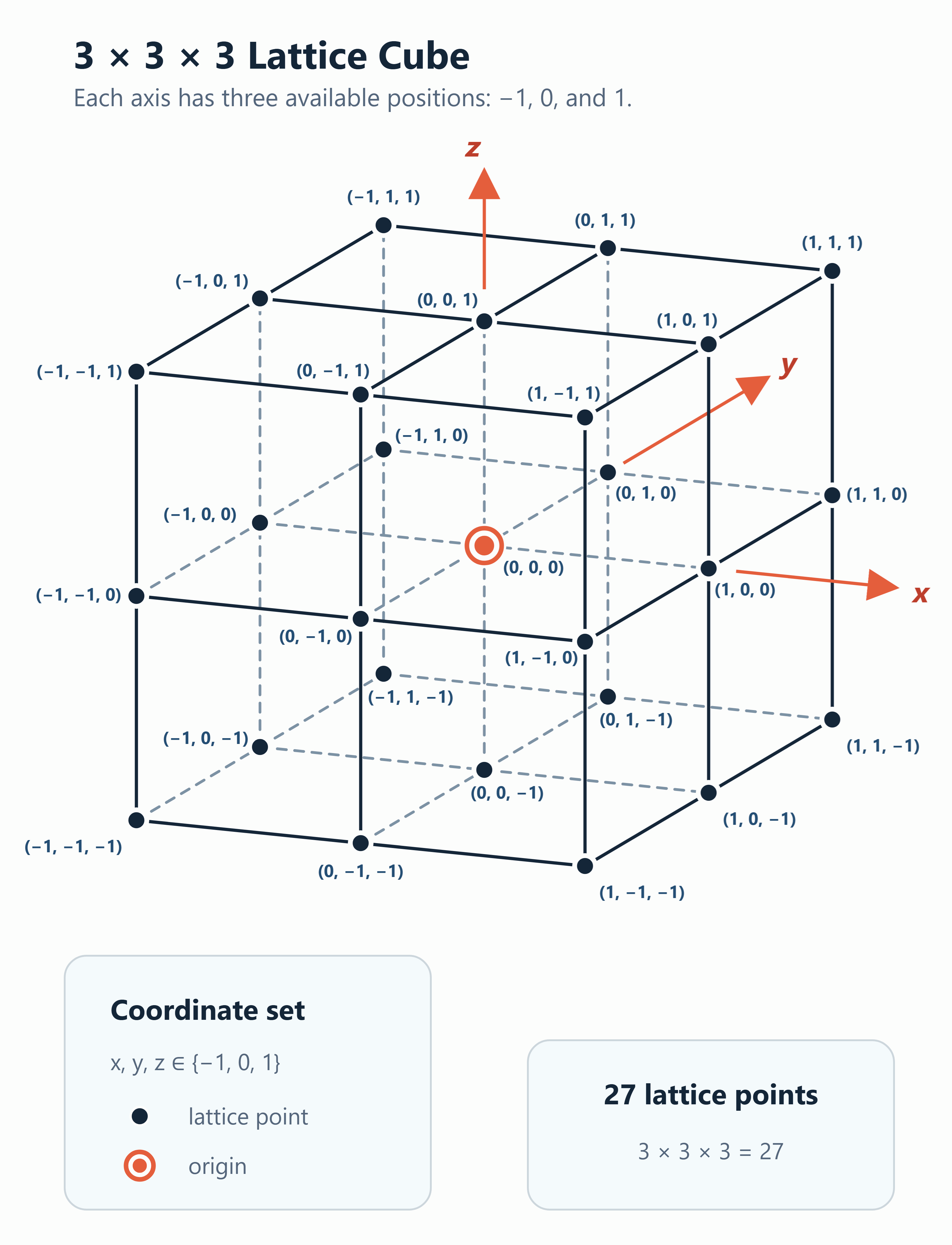
Figure 1. A 3 x 3 x 3 lattice cube. Each coordinate can take one of the three
values -1, 0, or 1.
Following this rule, 27 different points can be reached. Each axis provides
three states, so the total number of possible points is:
3(x) * 3(y) * 3(z) = 27
Now let us try the same idea with a lattice in six-dimensional space.
This time, we also increase the extent to three steps in either direction.
Each axis therefore allows the positions:
{-3, -2, -1, 0, 1, 2, 3}
There are seven possible positions on each of six axes. The complete
six-dimensional lattice therefore contains:
76 = 117,649 points
We can assign all these points to a two-dimensional square grid.
For such a square arrangement, the dimension of the original lattice
must be even: 2, 4, 6, 8, and so on. An even dimension makes this square
arrangement possible; an odd dimension does not produce such a square in this
form.
Let us examine this in more detail using the relation:
q2m = (qm)2
Here, q is the number of possible states on each axis. The lattice extends
equally far in the negative and positive directions, with zero as the central
state. If the extent in either direction is r, then q = 2r + 1, so q is always
odd. The value m is a positive integer, so 2m is the even dimension of the
original lattice.
As a result of this relation, the higher-dimensional lattice can be arranged
in the plane as a qm by qm square containing the same number of lattice
points. Since q is odd, the side length qm is odd as well. The square
therefore has one lattice point exactly at its center, and this point serves
as the origin.
Our six-dimensional object with seven possible positions on every axis has
the same property: the origin lies at the center of all the lattice points.
But how are the points assigned?
That is what the following example demonstrates.
## UNDERSTANDING THE METHOD THROUGH ONE EXAMPLE
We use a six-dimensional lattice with the following available coordinate
values:
{-3, -2, -1, 0, 1, 2, 3}
As our example, we choose the point:
P = [-3, 0, 1, -1, 3, -2]
### 1)
First, split the six components into two blocks of equal length:
Px = [-3, 0, 1]
Py = [-1, 3, -2]
Px will produce the horizontal coordinate in the 2D plane.
Py will produce the vertical coordinate.
Other arrangements are possible, but the chosen component order must remain
consistent throughout the transformation.
### 2)
For the moment, concentrate only on the first block:
Px = [-3, 0, 1]
### 3)
To convert the components, add the extent r to each component. In our example,
the extent is r = 3. Therefore:
digit = component + 3
This relation produces the following mapping:
component becomes digit
-3 -> 0
-2 -> 1
-1 -> 2
0 -> 3
1 -> 4
2 -> 5
3 -> 6
The first block therefore changes from:
Px = [-3, 0, 1]
to:
Px' = [0, 3, 4]
### 4)
Now take the three components in their existing order as a number:
034
### 5)
At this point, we need to treat 034 as a numeral in the base-7 numeral system.
We use base 7 because every axis has seven possible coordinate states.
This also makes the purpose of the digit range from 0 to 6 clear: the base-7
system permits exactly these seven digits. As shown in step 3, adding r shifts
the coordinate values from the range
{-r, ..., r} into the nonnegative digit range
{0, ..., 2r}. This is what makes the numeral-system
representation applicable.
Converting 034 from base 7 into a decimal number gives:
034(base 7)
= 0 * 72 + 3 * 71 + 4 * 70
= 0 + 21 + 4
= 25
**Specialized** In an array, positions are counted
starting from the left. In a number, place values are counted starting from the
right. To assign the positions of an array directly to the corresponding place
values of a number, the digit sequence must therefore be reversed: 034 becomes
430. In our example, we read 034 directly in the reading direction because
this makes the procedure easier to explain.
### 6)
The complete first coordinate block has now become one value:
Px'' = [25]
### 7)
Apply exactly the same procedure to:
Py = [-1, 3, -2]
Adding the extent r = 3 to each component, as in step 3, gives:
Py' = [2, 6, 1]
Read these digits as the base-7 number 261:
261(base 7)
= 2 * 72 + 6 * 71 + 1 * 70
= 98 + 42 + 1
= 141
Therefore:
Py'' = [141]
### 8)
Join the two resulting values to form a point in the 2D plane:
P'' = [25, 141]
At this stage, the assignment is complete, but the square grid is not yet
centered around the origin.
### 9)
The origin of the original six-dimensional lattice lies exactly at the center
of its extent. We now reproduce that centered arrangement in the 2D plane.
First calculate the side length of the square:
side length
= √ total number of points
= √(76)
= 73
= 343
There are 343 positions along each side. Because the positions are indexed
starting at 0, the first index is 0 and the last index is 343 - 1 = 342.
This does not mean that there are only 342 positions: counting both 0 and 342,
the range contains all 343 positions.
number of positions = 343
first index = 0
last index = 343 - 1 = 342
The central index lies halfway between the first and last indices:
centering value
= 342 / 2
= 171
Subtract this centering value from both components of P'':
P''' = [25 - 171, 141 - 171]
This shift removes the effect of starting the count at zero and creates a new
origin [0, 0] exactly in the center of the 2D square.
Complete the calculation to obtain the final result:
P''' = [-146, -30]
### 10)
THLP has now transformed the six-dimensional point:
P = [-3, 0, 1, -1, 3, -2]
into the two-dimensional point:
P''' = [-146, -30]
In compact form:
[-3, 0, 1, -1, 3, -2]
THLP
|
v
[-146, -30]
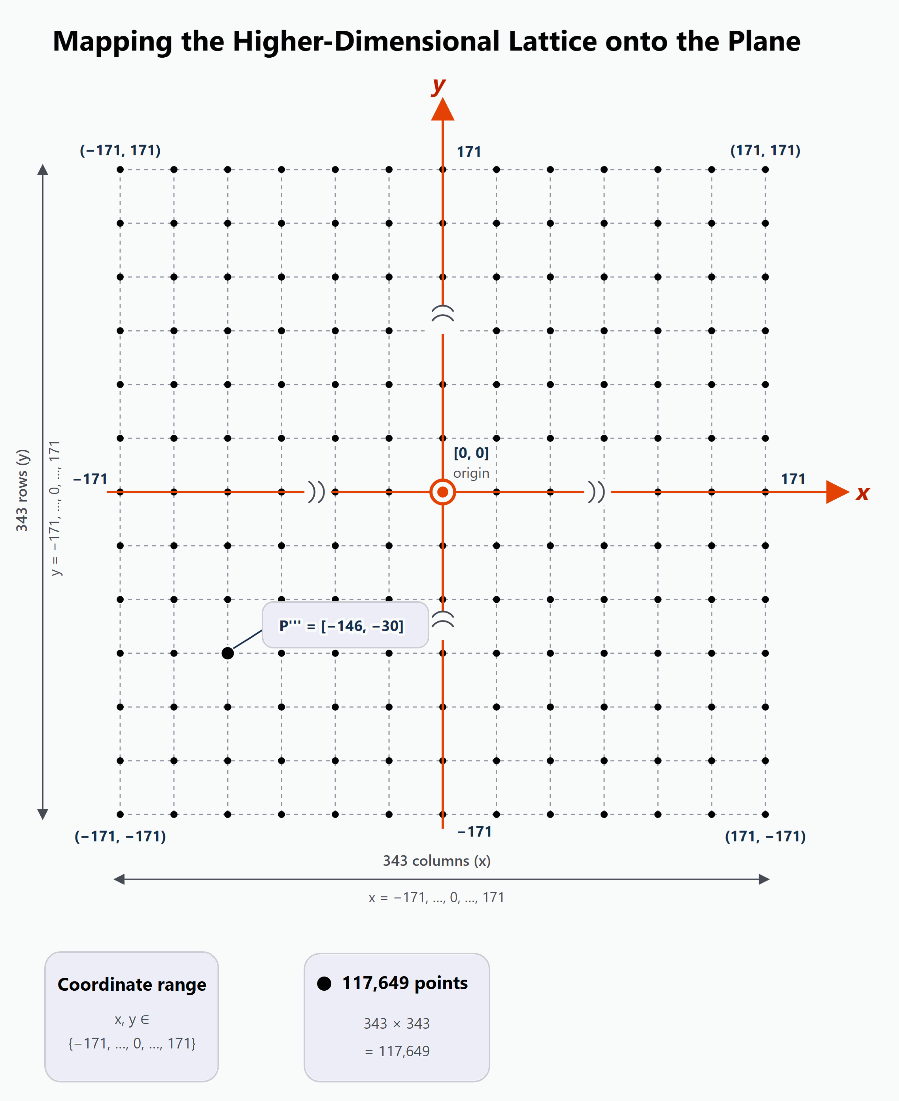
Figure 2. The transformed point on the centered 343 x 343 square grid.
The forward transformation is now complete.
## MAPPING THE PLANE BACK INTO HIGHER-DIMENSIONAL SPACE
To create the visualizations, we also need to apply the transformation in the
opposite direction. For every pixel or grid position in the image, we identify
the corresponding vector in the higher-dimensional lattice. A separate
visualization method can then use that vector to determine the color assigned
to the selected position.
The inverse transformation follows the previous procedure in reverse. We use
the same example, beginning with the point obtained in the plane:
P''' = [-146, -30]
### 1)
First, undo the centering operation by adding 171 to both coordinates:
P'' = [-146 + 171, -30 + 171]
= [25, 141]
### 2)
Convert each coordinate back into its previously used base-7 representation,
including the leading zero:
25 = 034(base 7)
141 = 261(base 7)
### 3)
Separate the digits to recover the two shifted coordinate blocks:
Px' = [0, 3, 4]
Py' = [2, 6, 1]
### 4)
Undo the shift from the forward transformation. Since the extent r = 3 was
added to each component before, we now subtract 3 from each digit:
component = digit - 3
Apply this inverse rule to both coordinate blocks:
Px' = [0, 3, 4]
-> Px = [0 - 3, 3 - 3, 4 - 3]
= [-3, 0, 1]
Py' = [2, 6, 1]
-> Py = [2 - 3, 6 - 3, 1 - 3]
= [-1, 3, -2]
### 5)
Join the two coordinate blocks in their original order:
P = [-3, 0, 1, -1, 3, -2]
The point in the centered plane has now been mapped back to its original
six-dimensional vector:
[-146, -30]
inverse THLP
|
v
[-3, 0, 1, -1, 3, -2]
This inverse assignment makes it possible to locate the higher-dimensional
vector associated with every position in the square. That vector can then
serve as the input for the chosen visualization method. This requires the
dimension and extent of the underlying lattice to be specified in advance and
kept unchanged throughout the assignment.
## HOW THE VISUALIZATIONS ARE CREATED
How can a color be assigned to each point on the basis of its corresponding
vector?
My first experiment used the vector's distance from the origin. The
Pythagorean theorem can be extended to any number of dimensions by adding the
squares of all vector components. For our example vector, this gives:
P = [-3, 0, 1, -1, 3, -2]
squared components
= [(-3)2, 02, 12, (-1)2, 32, (-2)2]
distance squared
= sum of the squared components
= 24
The actual Euclidean distance is therefore:
distance = √24
In a computer implementation, taking the square root is not necessary.
The squared distance already provides a value that can be used by a chosen
color rule. One possible rule is: if the calculation returns the value 24 for
a pixel, color that pixel green.
Applying such a rule to every position in the square produces the complete
visualization: each position is mapped back to its higher-dimensional vector,
and the chosen method calculates from that vector the value that determines
the color of the corresponding pixel.
One of the most powerful approaches was to compare the Px component block of
the higher-dimensional vector directly with its Py component block. In this
comparison, the components at the same position in the two blocks were matched
with each other. The relationships obtained from this component-by-component
comparison could then be translated into color values.
After reaching a first surprising result, one will probably be tempted to
experiment with many other rules. Those possibilities are not described here.
The visual results presented here differ considerably, yet they all share the
same underlying construction described in this text.
One further observation may be useful. Although both the extent and the
dimension affect the total number of lattice points, they often play
noticeably different visual roles. In my experiments, changing the extent
tended to alter the style and texture of the resulting image, whereas the
dimension primarily affected the area occupied by the depicted structure. This
may be the opposite of what one would initially expect.
In the Number Garden browser application, an identifier such as 3-NOR-2c is
displayed in the browser tab. Pressing the “F” key also displays it directly in
the application. The first number, 3 in this example, deserves particular
attention: it indicates the extent and has an especially strong influence on
the characteristic expression of the graph. This value applies in both the
positive and negative axis directions. An extent of 3 therefore comprises the
coordinate values {−3, −2, −1, 0, 1, 2, 3}. It is worth keeping an eye on this
first number and comparing its changes with the appearance of the generated
graphs.
The remainder of the identifier (NOR-2c in this example) provides additional
information about the visualization techniques used, which will not be
discussed further here. The dimension itself is not included in the identifier.
Its influence is most apparent in the area occupied by the forms. This becomes
especially clear when they are set in motion by tapping the display.
The distinctive spatial characteristics of the projection also tended to
become less pronounced as the extent increased. The visual signature of THLP
was therefore often clearest at smaller extents, although larger extents could
still produce surprising results. These are practical observations from the
visual experiments rather than strict mathematical rules.
## CLOSING REMARK
> **THLP creates an ordering principle – by balancing finite number spaces around a common origin.**
I have tried to describe the construction of these visualizations in enough
detail to make it understandable and reproducible, while keeping the
explanation focused without reducing it to the bare minimum.
The underlying principle is not necessarily limited to mapping into a
two-dimensional square. By dividing the source coordinates into a different
number of blocks, the same encoding idea can be used to map between other
dimensions. The method works in both directions. More generally, the method
could serve as a link between different dimensions.
With suitable additions, the method might also be extended to lattices with an
odd number of dimensions. This would require a suitable way to handle unequal
coordinate blocks or rectangular target structures.
Apart from all theory, while viewing these visualizations it may be worth
remembering that otherwise hidden secrets of space and extent are genuinely
revealed here.
## How THLP Came About
I am a computer hobbyist living in Switzerland, near Basel. I became fascinated by pattern generation, and that fascination led me to create Number Garden. The images it produced surprised and impressed me, while also raising questions whose exploration eventually led to THLP. Press the button at the very bottom. It opens www.Number-Garden.com with the suffix /?@THLP@, which unlocks THLP mode.
AI was used as an aid in programming and in preparing this article. The underlying structural properties of the patterns, as well as the discovery and development of THLP, are the result of my own human work and conception. This groundwork was essential: the aim was not to visualize arbitrary images, but to produce patterns through a strictly defined, human-verified computational process. It involved a great deal of my own work.